The GPGPU project was an investigation into general purpose computing on graphics processing units (GPGPU) programming by Ilari Shafer for Computer Architecture, Spring 2008. The project had a few primary goals:
- Describe GPGPU architecture - specifically, on the GeForce 8x series
- Use the NVIDIA Common Unified Device Architecture (CUDA) toolkit
- Implement a program on the CPU that lends itself to parallelization on the GPU
- Write a similar program that executes on the GPU
- Visualize the results and compare the speed to CPU execution time
This document is organized roughly into these sections. Feel free to use the table of contents at left to explore.
What is GPGPU?
The Origins of GPGPU
GPGPU stands for General Purpose computing on Graphics Processing Units, and refers to a type of multicore programming that has recently become much more approachable. This development has been driven in large part by changes in the architecture of GPUs. *
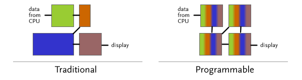
Traditional graphics cards have contained a rendering pipeline that was largely fixed: hardware would be devoted to tasks like geometric computation, lighting, and rasterization. This process is illustrated (very roughly) at left above - imagine that different colors represent different operations. However, as a multitude of 3D applications evolved, the usage of the various components varied. To allow for enhanced pipeline configurability and changing requirements on the software API side, programmable pipelines developed. First to arrive were programmable pixel and vertex shaders *; now, a typical GPU from ATI or NVIDIA has fully-programmable "stream-processing" units that can adopt any operation in the 3D pipeline - or even other tasks. This trend has allowed even consumer-level GPUs to perform as configurable multi-core processing units*, and manufacturers have released toolkits that allow developers to run code on the stream processors. GPUs are well-suited to highly data-parallel computation, often with floating-point math - operations like image processing, video encoding/decoding, and pattern recognition (see the CUDA gallery for more detail).
System Architecture
This document describes GPGPU in the context of the NVIDIA Geforce 8600 GTS and the Compute Unified Device Architecture (CUDA) toolkit, for the sole reason that it was the available hardware for developing the visualization described below. The detailed architecture of a programmable GPU varies significantly across manufacturers and video card families, and the precise details of hardware implementation are not fully disclosed by manufacturers. That said, a significant amount of architectural information related to the programming model of modern NVIDIA GPUs is widely available, and the fundamental programming model is the same for all CUDA devices.
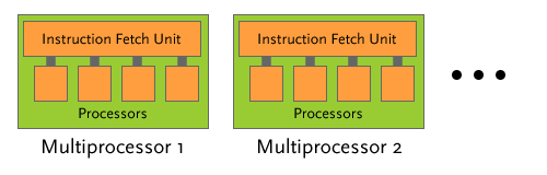
The diagram above (based on *, p. 16) shows the general hardware layout of a 8x series GPU. A number of "multiprocessors" (4 for the 8600 GTS) each have a number of cores (8) that execute the same instructions in parallel. In this sense, each "multiprocessor" can be seen as a SIMD unit - a typical program will issue instructions that are executed across different elements in memory. Each processor has a small set of registers, which allows it to maintain state information such as which block of data it operates on. In a significant deviation from CPU design, these processors operate with small caches and simple control units; GPUs have many more transistors devoted to data processing (see *, p. 3).
In general terms, work is scheduled in "blocks" of threads that are scheduled across the set of multiprocessors. Since CUDA software and hardware are responsible for running threads asynchronously from other code, there is an ability to synchronize threads by waiting for all currently-executing threads to complete*.
Programming Model
In order to distribute work across the multiprocessors described above, NVIDIA provides a C-based toolchain called CUDA. Fundamentally, CUDA attempts to exist as more-or-less device-independent layer between a "kernel" of code to execute and the details of how it is duplicated and distributed on the GPU.
Threading Model
CUDA encourages programmers to think of the hardware as a "single instruction, multiple thread" device. Pieces of parallel code called "kernels" are executed in multiple threads, which are further grouped into a number of blocks. A "grid" of blocks is run as a unit of computation on the GPU.
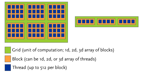
The diagram above (adapted from *, p. 9) illustrates how threads are grouped. Up to 512 individual threads can be grouped into a "block," either in a one-dimensional, two-dimensional, or three-dimensional array. Deciding which format to use is largely for the organizational convenience of the programmer. For example, when applying a function to 2D image data, a typical use seems to be to split threads into 2D blocks of, say, 16*16 (256 threads per block). This number is largely arbitrary (*, p. 7)/ Each thread executes its kernel on one pixel of image data; thus, a block will operate on a 16x16 piece of an image. Tiling blocks across the total image size will produce the appropriate operation.
Memory Architecture
Using memory on the GPU involves writing the interactions between host (CPU) and device (GPU) memory, as well as structuring memory access across the five different types of device memory. The GPU architecture employs a much smaller cache than a typical CPU, and also is heavily reliant on the spatial locality of reads. Careful memory access is the responsibility of the programmer.
The five different types of device memory are:
- Global memory: The largest available chunk of memory (somewhat smaller than 256MB of GDDR3 for the 8600GTS), and also the slowest. It is uncached, and the slowest memory store to access.
- Texture memory: A read-only segment of memory that is cached. The backing store lies in the same hardware as global memory. The cache is optimized for 2D spatial locality - sensible, considering its use in dealing with 2D textures.
- Constant memory: Another cached, read-only segment of memory that resides in the main memory of the GPU. It is accessed somewhat differently than texture memory, and is not optimized for 2D spatial locality.
- Shared memory: Faster memory that is shared across a block. In the image processing example above, all 256 threads could access this same chunk of memory. Kernel function parameters are stored here, and other data can be moved into shared memory using device code.
- Per-thread memory: Each thread a set of the registers associated with each block. However, "local" memory for the thread is actually stored in global memory, and accordingly is very slow.
Coordinating memory access between these different regions must be done by the programmer; the compiler can often not determine which memory region a pointer originates from. By way of example, attempting to use a double pointer as a kernel function parameter will result in a compiler warning and unexpected behavior, since the parameter itself is in shared memory, but may point to shared, texture, or constant memory. Debugging such errors is also difficult: when tested on the CUDA emulator, memory access may work smoothly, but when compiled to the different hardware memories of the device (where real-time debugging is not possible), accesses sometimes break.
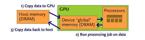
As shown above, a typical compute job begins by copying data to the GPU, usually to global memory. Instructions will also be copied to shared memory. The GPU then asynchronously runs the compute task it has been assigned. When the host makes a call to copy memory back to host memory (shown in step 3), the call will block until all threads have completed and the data is available, at which point results are sent back.
Special Syntax
To actually implement the threading and memory system above, CUDA includes a number of nonstandard extensions to C/C++. Programmers write code in .cu files, which are split and compiled to C++ for the host and C for the device, then compiled down to assembly. For more details on the compilation process, see *, p. 20.
First, a few new keywords mark functions and variables that exist in different locations on the host and device. A kernel function marked __device__ can only be executed on the device (and is inlined by default), whereas a kernel function marked __global__ can be invoked by the host to be executed on the device. Likewise, __host__ marks a function as executable only on the host CPU. The keywords __constant__ and __shared__ mark variables that exist in constant and shared memory, respectively. The lack of a modifier marks a variable as global; texture memory uses a special reference *.
The special reserved keywords blockIdx and threadIdx are 3-tuples of indices that refer to the index of the current thread on device code. For example, if we execute a kernel with block dimension (3, 2, 1) and grid dimension (2, 1, 1), we would produce 12 threads, split across two blocks. The threads would have threadIdx = (1, 1, 1), (2, 1, 1), etc.
__global__ void imkernel(int[] imagedata, int width, int height) {

     int x = blockIdx.x * blockDim.x + threadIdx.x;

     int y = blockIdx.y * blockDim.y + threadIdx.y;


     imagedata[y*width + x] |= 0x80808080;

}
The example above shows a generic (non-optimized) kernel that (crudely) brightens every pixel in an array. To see how the kernel is split across an image, envision the diagram from "threading model" superimposed on an image, with each blue thread operating on a single pixel.
To actually invoke a function executed on the device from the host, a special syntax describes the block and grid sizes that should be used for the kernel. A call to the above kernel would look like:
imkernel<<<grid, block>>>(imagedata, width, height);
Here, grid and block are the 3-tuple dimensions of a grid and block, respectively. They have the type dim3, which is simply a structure with x, y, and z components. Two additional arguments to the <<<>>> construct can specify a dynamic shared memory allocation and a data stream; see *, p. 23 for more detail.
Fractals on the CPU
To demonstrate the potential for high-performance parallel computation on the GPU, I chose an operation that appeared to lend itself well to GPU: animated fractal drawing. Each frame in an animation is independent and could be drawn by a separate core on the GPU, and could make heavy use of the native floating-point ALU on a GPU. I first implemented a fractal drawing program on the CPU to verify that I could understand the process and write the single-threaded C.
IFS Fractals
I chose to write a program that would draw Iterated Function System (IFS) fractals, a type of fractal that has a number of aesthetically pleasing forms and does not require extreme (i.e. double precision) floating-point math. One type of IFS fractals (so-called "fractal flames," is the basis for the popular Electric Sheep screensaver*. Unfortunately, generating these fractals involves a significant amount of coloration and investigation to find visually pleasing images.
The typical process of generating a 2D IFS fractal involves selecting a two-input, two-output function at random from a collection of functions and applying it to a point in the (x,y) plane, plotting the result, and repeating the process. A number of interesting fractals can be generated from a collection of simple linear transformations. The example shown below (in psuedocode) generates the Sierpinski Gasket in the domain 0<x<1, 0<y<1 *.
f[0] := (x, y) => (x/2, y/2)

f[1] := (x, y) => ((x+1)/2, y/2)

f[2] := (x, y) => (x/2, (y+1)/2)

(x, y) := (rand(), rand())

repeat many times:

    i := randomInteger(0, 2)

    (x, y) := f[i](x, y)

    plot(x, y)
To simplify an animation algorithm, I decided to only use IFS systems that had two functions, weighted with equal probability of selection. To represent the functions, I used a common technique, the affine transform, for representing 2D transformations. This transform can be represented by a simple 2x3 matrix:
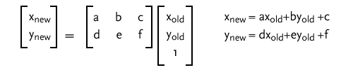
Finding values of a, b, c, d, e, and f, along with appropriate bounds on a window of x and y, that produce visually appealing images is still a process of trial and error. Much to my pleasure, a math professor* has already done the work of finding 188 such matrices and bounds*. Each .ifs file on the referenced gallery has matrix values for the two equiprobable affine transformations and a window size.
CPUFractal
I wrote an OpenGL/GLUT application to draw IFS fractals on the CPU. The implementation of a CPU-based, single-threaded CPU is provided in CPUFractal.exe, downloadable below. It uses a predefined list of fractal parameter files (from the gallery described above*), and interpolates linearly between matrices. This produces a continuous image of IFS fractals "reshaping" into other IFS fractals. The drawings are colored by the number of times a pixel is hit.
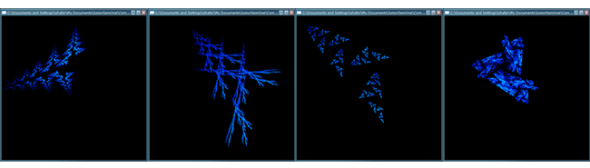
Shown above are some sample fractals produced by the program. The drawings are somewhat coarse and pixellated, since the image is not averaged over a number of samples. These fractals are generated from parameter files from the IFS gallery* in the "a" series.
The source code, Visual Studio project, and executable are provided below. CPUFractal.exe runs with no parameters. The project is a Visual Studio 2008 project, and has dependencies on GLUT and GLEW; to build, modify the additional include directories and linker path. The source files included are:
- CPUFractal.c: main program file
- util.h: random number generation
- affine.c/affine.h: single-frame IFS drawing code
- paramfile.c/paramfile.h: tools for loading and tweening IFS parameter files
- fileio.c/fileio.h: file list utilities
- sierpin.c/sierpin.h: draws the Sierpinski gasket

Fractals on the GPU
With a working implementation of IFS fractal drawing on the CPU, I wrote an implementation using CUDA on the GPU in an attempt to gain speed and unload the drawing computation from the CPU. Although the process of writing and debugging CUDA GPU code is unpleasant, a few utilities and approaches helped in developing the GPU fractal implementation. As described below, the GPU fractal implementation runs significantly faster than the CPU version, despite being relatively unoptimized and running on a single GeForce 8600 GTS.
Download Projects
The first step in running CUDA is obtaining an appropriate graphics card; a list of compatible cards is available here. Then, the CUDA toolkit must be installed. I used version 2.0, available from the CUDA download page. The CUDA SDK, available at the same location, is also extremely helpful for sample projects but is not required to develop with CUDA or run the code provided here.
Although the CUDA tools provide nearly everything needed to start developing a CUDA application, it is not transparent; starting from scratch is useful. In that spirit, I determined the subset of code that was necessary for writing a basic CUDA application. Due to the rather nonstandard compilation chain*, it is advisable to use a Visual Studio project file with external tools already set up. I wrote a Python script to create a blank project that contains a project file that will run the CUDA toolchain. The "GPU Projects" archive (downloadable below) contains:
- newproj.py: Run
python newproj.py [name]to create a new empty project with the name[name] - Blank: A blank project used by Python to copy and modify to create a new empty project. This project is a template for new projects; it should be modified only if the template needs to be changed.
- bin: Executables that are built from projects in the system are placed here.
- Debug: Used for the 32-bit "debug" target. Contains dlls that support GLUT/GLEW/CUDA executables.
- Release: For the 32-bit "Release" target. Also contains support libraries.
- EmuDebug: The CUDA toolkit has an emulator, which allows debugging of device to a certain extent. Using this target will create output here.
- common: Contains libraries and code for linking that is provided with the CUDA SDK and not with the CUDA toolkit.
- addarr: Contains source for
addarr, a simple test of CUDA. See Simple CUDA below for more detail. - texop: Contains source for
texop, an example of how to write to an OpenGL pixel unpack buffer. See GL+CUDA below for more detail. - fractal: Contains source for
fractal, the final GPU implementation. See GPU Fractal below for more detail.

Simple CUDA: addarr
To get started developing in CUDA, I wrote a simple program that uses the GPU to add a constant to each element of an array. The general execution flow occurs as shown in "Memory Architecture," and is illustrated in greater detail below.
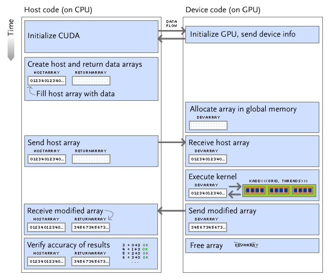
Note that all calls are initiated by the host, regardless of where they occur. The execution pathway I chose for addarr is similar to that chosen for most "general computation" tasks on the GPU:
- Send data and instructions to the device
- Run a computation on the device
- Wait for the computation to finish
- Copy the results back to the host
The simple test in addarr adds a constant to an array of numbers. This addition over n elements is parallelized over n threads grouped into blocks (of 512, for the GeForce 8600 GTS). The host checks that the GPU did indeed add the given number to each element successfully. All code is in addarr.cu.
GL + CUDA: texop
When developing a program that runs computation on the GPU and outputs it on a display, further load can be taken off the CPU and memory bus. For example, the GPU can run its computations on a OpenGL display buffer and the host can instruct OpenGL to display from the modified buffer.
I wrote texop.cu as a test of the buffer mapping mechanism. It also uses random numbers sent from the host, a resource that is necessary when computing IFS fractals. The execution flow is shown diagrammatically below.
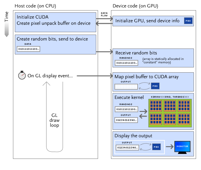
Unfortunately, the implementation of cudaGLMapBufferObject, the function that ostensibly maps an OpenGL buffer to a CUDA array*, is very slow. A call that should be merely a pointer assignment (or device-to-device copy, with bandwidth of 50-60GB/s) takes on the order of milliseconds for a 1MB array. Others have reported similar problems with the implementation (documented here).
GPU Fractal: fractal
Based on the implementation in CPUFractal and approach in texop, I wrote a CUDA/OpenGL program that generates the fractal animation on the GPU and displays it from a mapped pixel unpack buffer. The execution flow is substantially similar to that shown in texop: when OpenGL evaluates the display function (displayF), the GPU is instructed with CUDA to draw a particular IFS fractal in parallel then display it with OpenGL.
The fractal display is parallelized across 32 total threads in blocks of 4 threads. The grid size is chosen to be larger than 4 to be greater than the number of multiprocessors on the device: this allows the scheduler (in theory) to use all of the compute capability of the device to render a fractal. Notably, the parallelization of fractal computation is performed in a different manner than my first design.
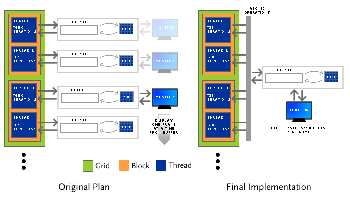
Originally, I wanted to run one grid of computation that would compute many frames of the fractal animation; one thread would compute one frame. This design has a few advantages: primarily, each thread could access a completely separate memory space, and there would be no synchronization problems with threads writing to the same locations in the frame buffer. Unfortunately, due to the amount of time required to map a buffer (discussed in texop above), this approach resulted in a significant delay when each kernel invocation was sent to the GPU.
Instead, fractal uses the architecture shown at right. The drawing kernel is invoked once per frame, and threads draw in parallel. Drawing IFS fractals is actually a very parallelizable task; if the original x and y coordinates and the indices of random function invocation are chosen from different random number sets for each thread (see the algorithm, above), the drawings can be overlaid. These different random numbers are implemented in fractal by using different portions of the randnos and randfloats arrays that are copied to the device.
One other precaution that must be taken for the architecture shown at right is thread data synchronization. Although it is unlikely that two threads will access the same memory location at once, the event still happens; since each pixel stores a "hit count," an incorrectly interleaved pair of += operations will cause instability in the resulting image. Fortunately, devices with "Compute Capability 1.1" (including the GeForce 8600 GTS) have atomic integer arithmetic operations. I use atomicAdd to guarantee data synchronization.
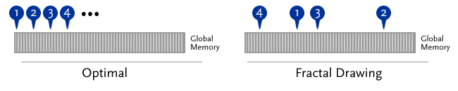
Unfortunately, one aspect of IFS fractal animation is not conducive to parallelization on a GPU: the memory access pattern. GPU access is highly optimized for spatial locality - for example, an algorithm that loops linearly through contiguous blocks of memory like the image algorithm shown in Special Syntax will be cached effectively *. However, IFS fractals require pixel counts at essentially random locations to be updated. The access pattern for fractal results in noncoalesced memory access*, as illustrated below.
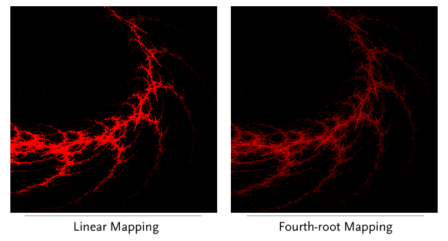
After drawing the fractal, the fractal program performs one additional step: using a GPU kernel to map the number of times a pixel is "hit" to a color in a nonlinear fashion. As documented in the flam3 algorithm*, using a logarithmic mapping can create a more visually pleasing fractal by highlighting the pixels that receive fewer hits. Instead of using a logarithmic map, I chose to use a (hits/256)1/4 map to the intensity of red color in the range [0, 1]. The kernel that implements this map (shown below) is highly parallelizable, and operates much faster than colormapping on the CPU, even when the CPU uses a precomputed colormap.
__global__ void mapcolors(outpointer op, int width, int height) {

     int x = blockIdx.x * blockDim.x + threadIdx.x;

     int y = blockIdx.y * blockDim.y + threadIdx.y;


     op.out[0][y*width+x] = (int)(sqrt(sqrt(

         (float) op.out[0][y*width+x] / 256.0

     ))*256.0);

}
Results
Colormapping
As described above, fractal uses a fourth-root map from number of pixel hits to color intensity. This mapping "draws out" more of the detail in the image without saturating the image. A comparison of the same fractal image with linear (red = hits * 8) and fourth-root (red = sqrt(sqrt(hits/256)) * 256) maps is shown below. As shown below in Speed Comparison, colormapping is much faster on the GPU than on the CPU.
Video
A video of one minute of the output produced by fractal is shown below. A series of "tweens" between different fractals found by Ken Brakke* is animated and displayed. Note that the quality shown in this video is much lower than that displayed on-screen; the video compression required of either available Flash codec (VP6 or H.263) produces many artifacts. The quality of the animated fractals is as shown in colormapping above. Download the GPU Fractal program and run it on a GeForce 8 series or higher GPU to see this animation.
Speed Comparison
To compare the speed of the CPU-based CPUFractal with the GPU-based fractal, I split off two functions: CPUFrame and GPUFrame, provided in fractal.cu (part of the fractal project). Each has the same signature: a number of iterations of the IFS algorithm to compute and a CUDA timer to use for logging how long portions of each function take. I ran both GPUFrame and CPUFrame for 307200 iterations per frame and averaged the timings over 1199 frames.
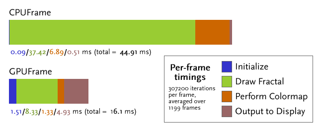
The timings above reflect an ≈2.8x speedup that results from computing IFS fractals in parallel on the GPU. A number of factors are important to consider in the timings above:
- The CPU used was a Core 2 Duo E7200, running at 2.53GHz with a 3MB cache, 1066MHz FSB, and 2GB of PC6400 RAM.
- The GPU used was a single GeForce 8600 GTS.
- Note the long "Initialize" and "Output to Display" times for the GPU. These represent the times taken for mapping and unmapping the OpenGL buffer. Clearly, the speed issues in
cudaGLMapBufferObjectandcudaGLUnmapBufferObjectdiscussed in GL + CUDA come into play. - The lack of coalesced memory access and concurrent memory access by multiple threads (potentially blocking on atomic operations) likely causes significant drops in performance.
Downloads
The binaries and source code for the GPU fractal program are available below. Note that these files are a subset of the projects collection above.

Conclusions
GPGPU is a technique that can unlock dramatic speed improvements in certain types of data-parallel computation. If a task and programmer can effectively exploit the multi-core design and many floating-point ALUs on the device, even an inexpensive consumer-level GPU can take work from the CPU to accelerate everyday tasks. Indeed, programs like a video encoder and a distributed protein-folding program are proven GPU-based products. That said, the paradigm is still in its infancy: the first OpenCL standard was released a week before this project was finished, and further developments are sure to come.
Computation of an IFS fractal animation on the GPU is eminently possible. Despite obstacles to parallelization like slow buffer map support and an algorithm that fundamentally does not access memory in a linear fashion, a 2.8x speedup can be attained on even a $30 graphics card. With better optimization of the algorithm and careful code profiling, further speed improvements could be realized. Additionally, visualization of parallelizable tasks on the GPU provides an excellent introduction to the types of disruptive changes possible with GPGPU.
Resources
References
- History of GPGPU. http://www.gpgpu.org/data/history.shtml
- Skadron, Kevin. Trends in Multicore Architecture. http://www.gpgpu.org/asplos2008/ASPLOS08-2-manycore.pdf
- 3D Pipeline Part II - Programmable shaders - To Infinity and Beyond. ExtremeTech. http://www.extremetech.com/article2/0,2845,1155161,00.asp
- CUDA Programming Guide Version 2.0. NVIDIA Corporation. 6/7/2008.
- NVIDIA CUDA Compute Unified Device Architecture Reference Manual, Version 2.0. June 2008
- The CUDA Compiler Driver NVCC. NVIDIA corporation. 4/1/2008.
- Dorache, Adrian. Blogs and C++ syntax highlighting. http://codecentrix.blogspot.com/2007/05/blogs-and-c-syntax-highlighting.html
- Draves, Scott and Reckase, Erik. The Fractal Flame Algorithm. http://flam3.com/flame.pdf
- Brakke, Ken. Iterated Function Systems. http://www.susqu.edu/brakke/IFS/default.htm
- Brakke, Ken. Gallery of IFS Images. http://www.susqu.edu/brakke/aux/IFS/gallery/gallery.htm
Thanks
- Mark Chang and the members of Computer Architecture, Spring 2008, for providing advice and guidance on the project
- Existing posts on CUDA Forums and the CUDA SDK for providing hints, workarounds, and existing approaches.
- Ken Brakke's IFS fractal gallery, for
.ifsfractal parameter files - Notepad2, for writing this page
- The MooTools framework, also for writing this page.
- The FamFam Silk Icons Set, for the file icons on this page.
- Blender, for creation of the opening animation